In this tutorial, you will learn how to forecast sales using machine learning and reinforcement learning.
To train machine learning models, we will use Linear Regression, Random Forest Regressor, and XGBoost Regressor algorithms. However, we will use LSTM based recurrent neural network to build a reinforcement learning model.
Finally, we will evaluate and compare the performance of all models on test data using various metrics including mean squared error, mean absolute error, and R2 score.
To build the models, we will use Store Item Demand Forecasting Data of 10 retail stores which is available from Kaggle. This tutorial will feature following tools/libraries to predict customer sales:
- Python
- Jupyter Notebook
- Scikit-Learn
- TensorFlow
- Keras
- pandas
- matplotlib
Article Contents
Article Notebook
Code: Customer Sales Prediction using Linear Regression, Random Forest, XG Boost, and LSTM
Prepared By: Awais Naeem (awais.naeem@embedded-robotics.com)
Copyrights: www.embedded-robotics.com
Disclaimer: This code can be distributed with the proper mention of the owner’s copyrights
Notebook Link: https://github.com/embedded-robotics/datascience/blob/master/customer_sales_prediction/sales_prediction_LR_XGB_RF_LSTM.ipynb
Store Item Demand Forecasting Dataset
This dataset contains around 913000 entries in the training dataset with each entry depicting the number of items sold at a particular store on daily basis from 2013 to 2017, inclusive.
Dataset Link:https://www.kaggle.com/competitions/demand-forecasting-kernels-only/data?select=train.csv
Input Data
- date: Date of the sale data. There are no holiday effects or store closures.
- store: Store ID
- item: Item ID
Output Data
sales: Number of items sold at a particular store on a particular date
Data Reading and Pre-Processing
Let’s first import all python-based libraries necessary to read/process the data and for building the machine learning models as well as the LSTM based recurrent neural network:
import os
import pandas as pd
import numpy as np
import matplotlib.pyplot as plt
from xgboost import XGBRegressor
from sklearn.ensemble import RandomForestRegressor
from sklearn.linear_model import LinearRegression
from sklearn.preprocessing import MinMaxScaler
from sklearn.metrics import mean_absolute_error, mean_squared_error, r2_score
from tensorflow.keras.models import Sequential
from tensorflow.keras.layers import Dense, LSTM
from tensorflow.keras.callbacks import EarlyStopping, ModelCheckpoint
Download the data set from the Kaggle website and place it in the home directory of the project. Now, you can read the dataset using Pandas read_csv function:
store_sales = pd.read_csv('store_sale.csv')
store_sales.head(10)
Output:
	  Date		store	item	sales
0	2013-01-01	1	1	13
1	2013-01-02	1	1	11
2	2013-01-03	1	1	14
3	2013-01-04	1	1	13
4	2013-01-05	1	1	10
5	2013-01-06	1	1	12
6	2013-01-07	1	1	10
7	2013-01-08	1	1	9
8	2013-01-09	1	1	12
9	2013-01-10	1	1	9
Firstly, let’s check if there are any null values in the dataset:
store_sales.info()
Output:
<class 'pandas.core.frame.DataFrame'>
RangeIndex: 913000 entries, 0 to 912999
Data columns (total 4 columns):
 #   Column  Non-Null Count   Dtype
---  ------  --------------   -----
 0   date    913000 non-null  object
 1   store   913000 non-null  int64
 2   item    913000 non-null  int64
 3   sales   913000 non-null  int64
dtypes: int64(3), object(1)
memory usage: 27.9+ MB
So, we have got 913000 rows of data with no NULL values in any of the columns. So far, so good…
Since we will deal with the overall sale of the items in all of the stores, we need to disregard the columns representing the Store ID and Item ID:
store_sales = store_sales.drop(['store','item'], axis=1)
The ‘date’ column in the dataset is of the ‘object’ datatype. So, we need to convert it to a DateTime datatype so that it can be used for further calculations:
store_sales['date'] = pd.to_datetime(store_sales['date'])
Rather than predicting the sales on the very next day, we will train the models to predict the sales in the next month. So, we need to convert our date to a period of ‘Month’ and then sum the number of items sold in each month:
store_sales['date'] = store_sales['date'].dt.to_period('M')
monthly_sales = store_sales.groupby('date').sum().reset_index()
To go back from ‘Period’ type to ‘DateTime’ type, we need to convert the resulting ‘date’ column to timestamp datatype:
monthly_sales['date'] = monthly_sales['date'].dt.to_timestamp()
monthly_sales.head(10)
Output:
date		sales
0	2013-01-01	454904
1	2013-02-01	459417
2	2013-03-01	617382
3	2013-04-01	682274
4	2013-05-01	763242
5	2013-06-01	795597
6	2013-07-01	855922
7	2013-08-01	766761
8	2013-09-01	689907
9	2013-10-01	656587
Now, we can visualize the monthly sales of the items as well:
plt.figure(figsize=(15,5))
plt.plot(monthly_sales['date'], monthly_sales['sales'])
plt.xlabel('Date')
plt.xlabel('Sales')
plt.title("Monthly Customer Sales")
plt.show()

Since our data is showing an increasing trend over time, we need to make this data stationary to improve the training phase of the learning models.
We can simply call the diff on the ‘sales’ columns to make our sale data stationery:
monthly_sales['sales_diff'] = monthly_sales['sales'].diff()
monthly_sales = monthly_sales.dropna()
monthly_sales.head(10)
Output:
date		sales	sales_diff
1	2013-02-01	459417	4513.0
2	2013-03-01	617382	157965.0
3	2013-04-01	682274	64892.0
4	2013-05-01	763242	80968.0
5	2013-06-01	795597	32355.0
6	2013-07-01	855922	60325.0
7	2013-08-01	766761	-89161.0
8	2013-09-01	689907	-76854.0
9	2013-10-01	656587	-33320.0
10	2013-11-01	692643	36056.0
plt.figure(figsize=(15,5))
plt.plot(monthly_sales['date'], monthly_sales['sales_diff'])
plt.xlabel('Date')
plt.xlabel('Sales')
plt.title("Monthly Customer Sales Diff")
plt.show()

Since we need to train our models to predict the sale of the items in the next month by looking at the sale of items in a specific number of previous months, we need to prepare a supervised dataset to feed into the machine learning model.
For this tutorial, we will keep the lookback number of months to be 12 i.e., previous 12-month sale data will be used to predict the sales in the successive 13th month.
Firstly, we need to drop off the ‘date’ and ‘sale’ columns in the dataset as we will be only dealing with the stationary sale data to train our machine learning model as well as the reinforcement learning model:
supverised_data = monthly_sales.drop(['date','sales'], axis=1)
Now, we need to prepare the supervised data such that the previous 12-month sale data is advertised as the input features and the 13th-month sale data is used as the output for the supervised learning models:
for i in range(1,13):
    col_name = 'month_' + str(i)
    supverised_data[col_name] = supverised_data['sales_diff'].shift(i)
supverised_data = supverised_data.dropna().reset_index(drop=True)
supverised_data.head(10)
Output:
sales_diff	month_1	month_2	month_3	month_4	month_5	month_6	month_7	month_8	month_9	month_10	month_11	month_12
0	3130.0	19380.0	-186036.0	36056.0	-33320.0	-76854.0	-89161.0	60325.0	32355.0	80968.0	64892.0	157965.0	4513.0
1	175184.0	3130.0	19380.0	-186036.0	36056.0	-33320.0	-76854.0	-89161.0	60325.0	32355.0	80968.0	64892.0	157965.0
2	84613.0	175184.0	3130.0	19380.0	-186036.0	36056.0	-33320.0	-76854.0	-89161.0	60325.0	32355.0	80968.0	64892.0
3	93963.0	84613.0	175184.0	3130.0	19380.0	-186036.0	36056.0	-33320.0	-76854.0	-89161.0	60325.0	32355.0	80968.0
4	23965.0	93963.0	84613.0	175184.0	3130.0	19380.0	-186036.0	36056.0	-33320.0	-76854.0	-89161.0	60325.0	32355.0
5	82168.0	23965.0	93963.0	84613.0	175184.0	3130.0	19380.0	-186036.0	36056.0	-33320.0	-76854.0	-89161.0	60325.0
6	-103414.0	82168.0	23965.0	93963.0	84613.0	175184.0	3130.0	19380.0	-186036.0	36056.0	-33320.0	-76854.0	-89161.0
7	-100472.0	-103414.0	82168.0	23965.0	93963.0	84613.0	175184.0	3130.0	19380.0	-186036.0	36056.0	-33320.0	-76854.0
8	-26241.0	-100472.0	-103414.0	82168.0	23965.0	93963.0	84613.0	175184.0	3130.0	19380.0	-186036.0	36056.0	-33320.0
9	41900.0	-26241.0	-100472.0	-103414.0	82168.0	23965.0	93963.0	84613.0	175184.0	3130.0	19380.0	-186036.0	36056.0
Now split this data into training and test data:
train_data = supverised_data[:-12]
test_data = supverised_data[-12:]
print('Train Data Shape:', train_data.shape)
print('Test Data Shape:', test_data.shape)
Output:
Train Data Shape: (35, 13)
Test Data Shape: (12, 13)
The next step is to scale the feature values to restrict them to a range of (-1,1) using MinMaxScaler():
scaler = MinMaxScaler(feature_range=(-1,1))
scaler.fit(train_data)
train_data = scaler.transform(train_data)
test_data = scaler.transform(test_data)
In the supervised DataFrame, first column corresponds to the output and the remaining columns act as the input features:
X_train, y_train = train_data[:,1:], train_data[:,0:1]
X_test, y_test = test_data[:,1:], test_data[:,0:1]
y_train = y_train.ravel()
y_test = y_test.ravel()
print('X_train Shape:', X_train.shape)
print('y_train Shape:', y_train.shape)
print('X_test Shape:', X_test.shape)
print('y_test Shape:', y_test.shape)
Output:
X_train Shape: (35, 12)
y_train Shape: (35,)
X_test Shape: (12, 12)
y_test Shape: (12,)
In the last step of data pre-processing, we will make a prediction data frame to merge the predicted sale prices of all the trained algorithms:
sales_dates = monthly_sales['date'][-12:].reset_index(drop=True)
predict_df = pd.DataFrame(sales_dates)
We also need to extract the actual monthly sale values of the last 13 months since they correspond to test data set. These values will later be used to find the predicted sale prices from the predicted output of sale difference via trained models:
act_sales = monthly_sales['sales'][-13:].to_list()
Now we are done with the core part of processing the data and preparing it to be used by the models. Next, we just need to train the algorithms on the training data and evaluate them on the testing data.
So, let’s get to the fun part…
Forecast Sales using Linear Regression
Linear Regression tries to find a linear relationship between a set of input variables and the output variable.
Weights attached with the input variables are updated during the training phase so that the predicted output aligns well with the desired output.
To train Linear Regression, we can simply call it using scikit-learn and pass the training data. Moreover, we can use the ‘predict’ function of the linear regression model to get the predicted outputs using the test data:
linreg_model = LinearRegression()
linreg_model.fit(X_train, y_train)
linreg_pred = linreg_model.predict(X_test)
To transform the predicted values back to their original scale, we need to call the ‘inverser_transform’ function of the MinMaxScaler. For that, we need to create a test set matrix containing all the input features of the test data and the predicted output instead of the real output:
linreg_pred = linreg_pred.reshape(-1,1)
linreg_pred_test_set = np.concatenate([linreg_pred,X_test], axis=1)
linreg_pred_test_set = scaler.inverse_transform(linreg_pred_test_set)
Once we have restored the scale of the predicted output for the sale difference, we need to calculate the predicted sale values from the difference values and append that to the predicted data frame which we created earlier:
result_list = []
for index in range(0, len(linreg_pred_test_set)):
    result_list.append(linreg_pred_test_set[index][0] + act_sales[index])
linreg_pred_series = pd.Series(result_list,name='linreg_pred')
predict_df = predict_df.merge(linreg_pred_series, left_index=True, right_index=True)
Since we have calculated predicted sale values for the test data, we can now evaluate various metrics for the trained Linear Regression model by comparing the predicted sale values with the actual sale values:
linreg_rmse = np.sqrt(mean_squared_error(predict_df['linreg_pred'], monthly_sales['sales'][-12:]))
linreg_mae = mean_absolute_error(predict_df['linreg_pred'], monthly_sales['sales'][-12:])
linreg_r2 = r2_score(predict_df['linreg_pred'], monthly_sales['sales'][-12:])
print('Linear Regression RMSE: ', linreg_rmse)
print('Linear Regression MAE: ', linreg_mae)
print('Linear Regression R2 Score: ', linreg_r2)
Output:
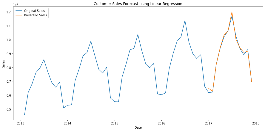
Linear Regression RMSE:  16221.272385416856
Linear Regression MAE:  12433.184266490774
Linear Regression R2 Score:  0.9906152516380969
The model looks pretty fine in predicting the sale values. Let’s visualize the predictions against the actual values:
plt.figure(figsize=(15,7))
plt.plot(monthly_sales['date'], monthly_sales['sales'])
plt.plot(predict_df['date'], predict_df['linreg_pred'])
plt.title("Customer Sales Forecast using Linear Regression")
plt.xlabel("Date")
plt.ylabel("Sales")
plt.legend(["Original Sales", "Predicted Sales"])
plt.show()

Forecast Sales using Random Forest Regressor
Random Forest is an ensemble of decision trees in which the final output value is guided by the average of the outputs of all the decision trees making up the Random Forest model.
We can specify the number of decision trees using ‘n_estimators’ and the maximum depth per decision tree using ‘max_depth’. Once we have specified the parameters of the Random Forest, we can then fit the model on the training data and predict the output sale difference values:
rf_model = RandomForestRegressor(n_estimators=100, max_depth=20)
rf_model.fit(X_train, y_train)
rf_pred = rf_model.predict(X_test)
Now we need to revert the original scale of the predicted sale values using the ‘inverse_transform’ function of the MinMaxScaler():
rf_pred = rf_pred.reshape(-1,1)
rf_pred_test_set = np.concatenate([rf_pred,X_test], axis=1)
rf_pred_test_set = scaler.inverse_transform(rf_pred_test_set)
Once we have got the predicted sale difference values, we need to convert these values to the predicted sale amount and merge these values in the predicted data frame:
result_list = []
for index in range(0, len(rf_pred_test_set)):
    result_list.append(rf_pred_test_set[index][0] + act_sales[index])
rf_pred_series = pd.Series(result_list, name='rf_pred')
predict_df = predict_df.merge(rf_pred_series, left_index=True, right_index=True)
Now, we can evaluate the model metrics by comparing the predicted sale amount with the actual sale value:
rf_rmse = np.sqrt(mean_squared_error(predict_df['rf_pred'], monthly_sales['sales'][-12:]))
rf_mae = mean_absolute_error(predict_df['rf_pred'], monthly_sales['sales'][-12:])
rf_r2 = r2_score(predict_df['rf_pred'], monthly_sales['sales'][-12:])
print('Random Forest RMSE: ', rf_rmse)
print('Random Forest MAE: ', rf_mae)
print('Random Forest R2 Score: ', rf_r2)
Output:
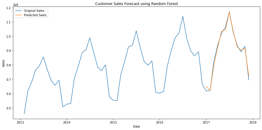
Random Forest RMSE:  17694.87898191384
Random Forest MAE:  14944.624166666696
Random Forest R2 Score:  0.9880636019264113
To visualize the predicted sale values against the actual sale of the items, we can plot the actual sale values and the predicted sale amounts for the test data as follows:
plt.figure(figsize=(15,7))
plt.plot(monthly_sales['date'], monthly_sales['sales'])
plt.plot(predict_df['date'], predict_df['rf_pred'])
plt.title("Customer Sales Forecast using Random Forest")
plt.xlabel("Date")
plt.ylabel("Sales")
plt.legend(["Original Sales", "Predicted Sales"])
plt.show()

Forecast Sales using XGBoost Regressor
XG Boost algorithm is the gradient boosting algorithm in which the effects of one decision tree are used to specify the learning parameters of the next decision tree unless the last decision tree generates a final output value.
The final output value is actually an ensembled value of all the decision trees included in the XGBoost regressor. We can specify the number of decision trees using ‘n_estimators’ and the learning rate of each decision tree using ‘learning_rate’:
xgb_model = XGBRegressor(n_estimators=100, learning_rate=0.2, objective='reg:squarederror')
xgb_model.fit(X_train, y_train)
xgb_pred = xgb_model.predict(X_test)
Once we have the predictions of sale difference, we need to convert these predictions back to their original scale:
xgb_pred = xgb_pred.reshape(-1,1)
xgb_pred_test_set = np.concatenate([xgb_pred,X_test], axis=1)
xgb_pred_test_set = scaler.inverse_transform(xgb_pred_test_set)
Now the last step is to convert unscaled sale difference predictions to item sale predictions and append the result to predict data frame:
result_list = []
for index in range(0, len(xgb_pred_test_set)):
    result_list.append(xgb_pred_test_set[index][0] + act_sales[index])
xgb_pred_series = pd.Series(result_list, name='xgb_pred')
predict_df = predict_df.merge(xgb_pred_series, left_index=True, right_index=True)
We can evaluate the performance of the XGB Regressor on the test dataset using various metrics:
xgb_rmse = np.sqrt(mean_squared_error(predict_df['xgb_pred'], monthly_sales['sales'][-12:]))
xgb_mae = mean_absolute_error(predict_df['xgb_pred'], monthly_sales['sales'][-12:])
xgb_r2 = r2_score(predict_df['xgb_pred'], monthly_sales['sales'][-12:])
print('XG Boost RMSE: ', xgb_rmse)
print('XG Boost MAE: ', xgb_mae)
print('XG Boost R2 Score: ', xgb_r2)
Output:
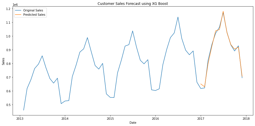
XG Boost RMSE:  15701.124706426719
XG Boost MAE:  13342.738751299059
XG Boost R2 Score:  0.9907513141349301
Let’s also visualize how out predicted sales stand against the actual sales in the last 12 months:
plt.figure(figsize=(15,7))
plt.plot(monthly_sales['date'], monthly_sales['sales'])
plt.plot(predict_df['date'], predict_df['xgb_pred'])
plt.title("Customer Sales Forecast using XG Boost")
plt.xlabel("Date")
plt.ylabel("Sales")
plt.legend(["Original Sales", "Predicted Sales"])
plt.show()

Forecast Sales using LSTM RNN
LSTM model consists of multiple layers, each one taking input from the previous one and advancing output to the next one. The first layer takes the numerical sequences as input, and the last layer gives the prediction value as the output.
We can define a sequential () model to embed the layers of LSTM. Later, we add an LSTM layer with 4 units followed by a fully connected hidden layer and an output layer.
The model will be compiled using the ‘adam’ optimizer to minimize the mean squared error by tweaking the weights during the training phase.
model = Sequential()
model.add(LSTM(4, batch_input_shape=(1, X_train_lstm.shape[1], X_test_lstm.shape[2])))
model.add(Dense(10, activation='relu'))
model.add(Dense(1))
model.compile(loss='mean_squared_error', optimizer='adam')
Before the training, we need to specify the number of epochs for which the network needs to be trained. Since we can’t be dead sure about the number of epochs, we need to specify the callback for EarlyStopping(), which will halt the model training after the model fails to minimize the validation loss value after the stated no. of epochs in the callback parameters.
checkpoint_filepath = os.getcwd()
model_checkpoint_callback = ModelCheckpoint(filepath=checkpoint_filepath, save_weights_only=False, monitor='val_loss', mode='min', save_best_only=True)
callbacks = [EarlyStopping(patience=5), model_checkpoint_callback]
Along with the callback for EarlyStopping(), you can specify the ModelCheckpoint() to monitor the loss after each epoch and save the best model in terms of validation loss.
Now, we will fit our model on the training data for a maximum of 200 epochs. Since we have specified the callback to monitor the loss on the validation dataset, we need to specify the validation data as well.
If the validation loss of the model is not minimized for five consecutive epochs, the training of the model will halt as specified in the callback.
history = model.fit(X_train_lstm, y_train, epochs=200, batch_size=1, validation_data=(X_test_lstm, y_test), callbacks=callbacks)
After the model training, it was observed that the model training was halted after 74 epochs because the validation loss did not improve after the 70th epoch.
Since we saved the model params in the ‘history’ variable, we can visualize the training/testing data loss:
metrics_df = pd.DataFrame(history.history)
print(metrics_df)
Output:
        loss        val_loss
0   0.307342  0.333725
1   0.283776  0.313256
2   0.266006  0.293502
3   0.250661  0.276005
4   0.234442  0.257560
..       ...       ...
69  0.003751  0.005788
70  0.003331  0.005641
71  0.003342  0.005622
72  0.003287  0.005677
73  0.003343  0.005778
We can also visualize the loss for training/testing data over the number of epochs using matplotlib:
plt.figure(figsize=(10,5))
plt.plot(metrics_df.index, metrics_df.loss)
plt.plot(metrics_df.index, metrics_df.val_loss)
plt.title('Sales Forecast Model Loss over Epochs')
plt.xlabel('Epochs')
plt.ylabel('Mean Squared Error')
plt.legend(['Training Loss', 'Validation Loss'])
plt.show()

Since we are done training our LSTM model on the training data, we need to predict the sale difference on the test data, upscale it to the original scale and then calculate the predicted item sale values:
lstm_pred = model.predict(X_test_lstm, batch_size=1)
lstm_pred = lstm_pred.reshape(-1,1)
lstm_pred_test_set = np.concatenate([lstm_pred,X_test], axis=1)
lstm_pred_test_set = scaler.inverse_transform(lstm_pred_test_set)
result_list = []
for index in range(0, len(lstm_pred_test_set)):
    result_list.append(lstm_pred_test_set[index][0] + act_sales[index])
lstm_pred_series = pd.Series(result_list, name='lstm_pred')
predict_df = predict_df.merge(lstm_pred_series, left_index=True, right_index=True)
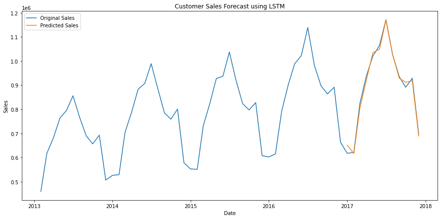
Now, we can evaluate the performance of the LSTM model on the test dataset and plot the predicted item sale values for the last 12 months of the test dataset:
lstm_rmse = np.sqrt(mean_squared_error(predict_df['lstm_pred'], monthly_sales['sales'][-12:]))
lstm_mae = mean_absolute_error(predict_df['lstm_pred'], monthly_sales['sales'][-12:])
lstm_r2 = r2_score(predict_df['lstm_pred'], monthly_sales['sales'][-12:])
print('LSTM RMSE: ', lstm_rmse)
print('LSTM MAE: ', lstm_mae)
print('LSTM R2 Score: ', lstm_r2)
Output:
LSTM RMSE:  15494.296868853291
LSTM MAE:  12533.464960899204
LSTM R2 Score:  0.9911825545326522
plt.figure(figsize=(15,7))
plt.plot(monthly_sales['date'], monthly_sales['sales'])
plt.plot(predict_df['date'], predict_df['lstm_pred'])
plt.title("Customer Sales Forecast using LSTM")
plt.xlabel("Date")
plt.ylabel("Sales")
plt.legend(["Original Sales", "Predicted Sales"])
plt.show()

Comparing Forecast Sales using Machine Learning Algorithms
As we have predicted the sales of items by training four different models, let’s compare the performance of all the models in terms of Root Mean Squared Error, Mean Absolute Error and R2 Score:
linreg_stats = [linreg_rmse, linreg_mae, linreg_r2]
rf_stats = [rf_rmse, rf_mae, rf_r2]
xgb_stats = [xgb_rmse, xgb_mae, xgb_r2]
lstm_stats = [lstm_rmse, lstm_mae, lstm_r2]
plt.figure(figsize=(15,7))
plt.plot(linreg_stats)
plt.plot(rf_stats)
plt.plot(xgb_stats)
plt.plot(lstm_stats)
plt.title("Model Comparison between Linear Regression, Random Forest, XG Boost and LSTM")
plt.xticks([0,1,2], labels=['RMSE','MAE','R2 Score'])
plt.legend(["Linear Regression", "Random Forest", "XG Boost", "LSTM"])
plt.show()

From the comparison curves for 3 metrics, LSTM performs overall best closely followed by XG Boost and Linear Regression. Random Forest seems a little bit off compared to other models but its performance can be tuned using hyperparameter optimization.
Conclusion
In this tutorial, we trained Linear Regression, Random Forest, XG Boost, and LSTM models to forecast the number of items sold for a successive month after taking input the sale data of the previous 12 months. Trained models were evaluated using Root Mean Squared Error, Mean Absolute Error, and R2 Score between the predicted sale values and the actual sale values in the test dataset.
All the models were able to predict the customer sales with an average root mean squared error of around 17000, mean absolute error of around 13500, and R2 score of around 0.99. All the models were built as a proof of concept to forecast sale predictions and no optimizations were performed to improve their performance. This tutorial showed that we can use machine learning and reinforcement learning algorithms to forecast sales predictions which can be really helpful to customize their budgets accordingly.

He is the owner and founder of Embedded Robotics and a health based start-up called Nema Loss. He is very enthusiastic and passionate about Business Development, Fitness, and Technology. Read more about his struggles, and how he went from being called a Weak Electrical Engineer to founder of Embedded Robotics.

Subscribe for Latest Articles
Don't miss new updates on your email!