How to perform Data Analysis and Visualization like a pro

Sharing is Caring!

This tutorial will deal with the data analysis and visualization of the video game sales dataset and try to extract useful insights from the data itself. These insights may prove useful for game publishers or platforms in taking crucial business decisions considering the sales worldwide.

The following tools/libraries will be used in this tutorial:

• Python
• Jupyter Notebook
• scikit-learn
• pandas
• NumPy
• matplotlib

Let’s firstly explore different parts of the video game sales data…

Article Notebook

Code: Data Analysis and Visualization using Video Game Sales Data Set

Prepared By: Awais Naeem (awais.naeem@embedded-robotics.com)

Copyrights: www.embedded-robotics.com

Disclaimer: This code can be distributed with the proper mention of the owner’s copyrights

Notebook Link: https://github.com/embedded-robotics/datascience/blob/master/video_game_data_analysis/video_game_data_analytics.ipynb

Video Game Sales Dataset

This dataset contains a list of video games with sales greater than 100,000 copies. There are a total of 16598 records with each record indicating the sales of a game in North America, Europe, Japan and in the rest of the world.

Wine Dataset Link: https://www.kaggle.com/datasets/gregorut/videogamesales

Data Features

Each record contains the following features in the video game sales dataset:

• Rank: Ranking of overall sales
• Name: Game Name
• Platform: Platform of the game release (e.g., PC, PS4, etc.)
• Year: Year of the game’s release
• Genre: Genre of the game
• Publisher: Publisher of the game
• NA_Sales: Sales in North America (in millions)
• EU_Sales: Sales in Europe (in millions)
• JP_Sales: Sales in Japan (in millions)
• Other_Sales: Sales in the rest of the world (in millions)
• Global_Sales: Total worldwide sales (in millions)

Data Reading

Let’s first import all python-based libraries necessary to read the data and for further pre-processing:

import numpy as np
import pandas as pd
import matplotlib.pyplot as plt

Since the data is given in a ‘csv’ format, we need to read it using the standard read_csv() function of pandas. We also need to specify the ‘rank’ column as the index of the dataframe:

vg_sales = pd.read_csv('video_game_sales.csv', index_col='Rank')
vg_sales.head()

Output:

        Name	Platform	Year	Genre	Publisher	NA_Sales	EU_Sales	JP_Sales	Other_Sales	Global_Sales
Rank 
1	Wii Sports	Wii	2006.0	Sports	Nintendo	41.49	29.02	3.77	8.46	82.74
2	Super Mario Bros.	NES	1985.0	Platform	Nintendo	29.08	3.58	6.81	0.77	40.24
3	Mario Kart Wii	Wii	2008.0	Racing	Nintendo	15.85	12.88	3.79	3.31	35.82
4	Wii Sports Resort	Wii	2009.0	Sports	Nintendo	15.75	11.01	3.28	2.96	33.00
5	Pokemon Red/Pokemon Blue	GB	1996.0	Role-Playing	Nintendo	11.27	8.89	10.22	1.00	31.37

Next, we need to make sure that there are no NULL values in the dataset. We can get an overall idea about the dataset using the info() method of the dataframe:

vg_sales.info()

Output:

<class 'pandas.core.frame.DataFrame'>
Int64Index: 16598 entries, 1 to 16600
Data columns (total 10 columns):
 #   Column        Non-Null Count  Dtype  
---  ------        --------------  -----  
 0   Name          16598 non-null  object 
 1   Platform      16598 non-null  object 
 2   Year          16327 non-null  float64
 3   Genre         16598 non-null  object 
 4   Publisher     16540 non-null  object 
 5   NA_Sales      16598 non-null  float64
 6   EU_Sales      16598 non-null  float64
 7   JP_Sales      16598 non-null  float64
 8   Other_Sales   16598 non-null  float64
 9   Global_Sales  16598 non-null  float64
dtypes: float64(6), object(4)
memory usage: 1.4+ MB

From the above information, we can clearly see that there are some NULL values present in the Year and Publisher columns. So, we are better off deleting the rows containing the NULL values for either the Year or the Publisher:

vg_sales = vg_sales.dropna(axis=0).reset_index(drop=True)

Since we are only going to extract useful insights from the data and not going to train any machine learning algorithm on this dataset, we only need this much pre-processing. Let’s now advance to analyze datasets and draw interactive visualizations.

Data Analysis and Visualization

For an exploratory data analysis, we will individually consider the sales for each of the Platform, Year, Genre and Publisher. Moreover, we will analyze the sales by combining two features i.e., platform yearly sales, genre yearly sales, platform sales by genre, etc.

Such an approach will allow us to explore and analyze each aspect of the data. Since we have the data for a large number of platforms, genre and publishers, we will consider only the top few in the context of sales for our analysis. However, analysis could be extended to any number of platforms, genre or publishers using the analysis and visualization techniques discussed in this article.

Let’s first analyze the sales in the context of platform:

Platform Sales

To calculate the sales of each platform, we need to group the dataframe using the ‘Platform’ column and then take the sum of all the values in a single group. This will produce a dataframe with each platform as the unique index and the cumulative values of all the numeric features in their respective columns for each platform.

Once we have done so, we can extract the columns related to the sales of each platform and organize the platforms from highest to lowest global sales:

platform_sales = vg_sales.groupby(['Platform']).sum().sort_values('Global_Sales', ascending=False)[['NA_Sales', 'EU_Sales', 'JP_Sales', 'Other_Sales', 'Global_Sales']]
platform_sales.head()

Output:

	               NA_Sales	EU_Sales	JP_Sales	Other_Sales	Global_Sales
Platform
PS2	572.92	332.63	137.54	190.47	1233.46
X360	594.33	278.00	12.30	84.67	969.60
PS3	388.90	340.47	79.21	140.81	949.35
Wii	497.37	264.35	68.28	79.20	909.81
DS	388.53	194.05	175.02	60.29	818.91

As the top 10 platforms hold the majority of the market, we will now visualize the market share of these platforms by examining the sales in North America, Europe, Japan, and the rest of the world:

platform_dum_values = np.arange(0, len(platform_sales.index[:10])*2, 2)
bar_width = 0.3
plt.figure(figsize=(20,10))
plt.bar(platform_dum_values, platform_sales['Global_Sales'][0:10], width=bar_width, label='Global Sales')
plt.bar(platform_dum_values+bar_width, platform_sales['NA_Sales'][0:10], width=bar_width, label='NA Sales')
plt.bar(platform_dum_values+(bar_width*2), platform_sales['EU_Sales'][0:10], width=bar_width, label='EU Sales')
plt.bar(platform_dum_values+(bar_width*3), platform_sales['JP_Sales'][0:10], width=bar_width, label='JP Sales')
plt.bar(platform_dum_values+(bar_width*4), platform_sales['Other_Sales'][0:10], width=bar_width, label='Other Sales')
plt.xticks(platform_dum_values + (bar_width * (len(platform_sales.columns)-1)/2), labels=platform_sales.index[:10])
plt.title('Video Game Sales (in millions) by Platform')
plt.xlabel('Platform')
plt.ylabel('Sales (millions)')
plt.legend()
plt.show()

Looking at the above plot, we can extract the following business insights related to the sales of the top ten platforms:

• First and foremost, 8 out of 10 platform have more sales in North America compared to Europe, Japan or the rest of world. So, any platform looking to increase their sales should concentrate marketing efforts in North America. Also, any new platform intending to enter into video game market should firstly target North America as its inhabitants seem to be gaming savvy
• Sales in Europe come next to those of North America for most of the platforms. So, if any platform has already got its market share in North America, next target location should be Europe
• PC, PS4 and X360 platform sales are extremely low in Japan compared to the rest of the locations. This should be a worrying sign for each of these platforms. The major reason for this discrepancy could be gaming interest of the Japanese people or non-serious marketing efforts in this region
• DS, PS and GBA platforms have much more sales in Japan than the rest of the world. These platform manufacturers need to look at the scalability of their produce in the rest of the world rather than just focusing on the North America, Europe and Japan

Yearly Sales

To calculate yearly sales, we need to group the video game data frame (vg_sales) by year and then take the sum of the sales for each unique year. For this scenario, we will not sort our data based on global sales but we will keep it sorted using the year.

yearly_sales = vg_sales.groupby(['Year']).sum()[['NA_Sales', 'EU_Sales', 'JP_Sales', 'Other_Sales', 'Global_Sales']]
yearly_sales.head()

Output:

	              NA_Sales	EU_Sales	JP_Sales	Other_Sales	Global_Sales
	Year			
1980.0	10.59	0.67	0.00	0.12	11.38
1981.0	33.40	1.96	0.00	0.32	35.77
1982.0	26.92	1.65	0.00	0.31	28.86
1983.0	7.76	0.80	8.10	0.14	16.79
1984.0	33.28	2.10	14.27	0.70	50.36

Now we will draw a line chart over the complete timeframe to see sales trend over time:

plt.figure(figsize=(20,10))
plt.plot(yearly_sales.index, yearly_sales['Global_Sales'], label='Global Sales')
plt.plot(yearly_sales.index, yearly_sales['NA_Sales'], label='NA Sales')
plt.plot(yearly_sales.index, yearly_sales['EU_Sales'], label='EU Sales')
plt.plot(yearly_sales.index, yearly_sales['JP_Sales'], label='JP Sales')
plt.plot(yearly_sales.index, yearly_sales['Other_Sales'], label='Other Sales')
plt.title('Video Game Sales (in millions) by Year')
plt.xlabel('Year')
plt.ylabel('Sales (millions)')
plt.legend()
plt.show()

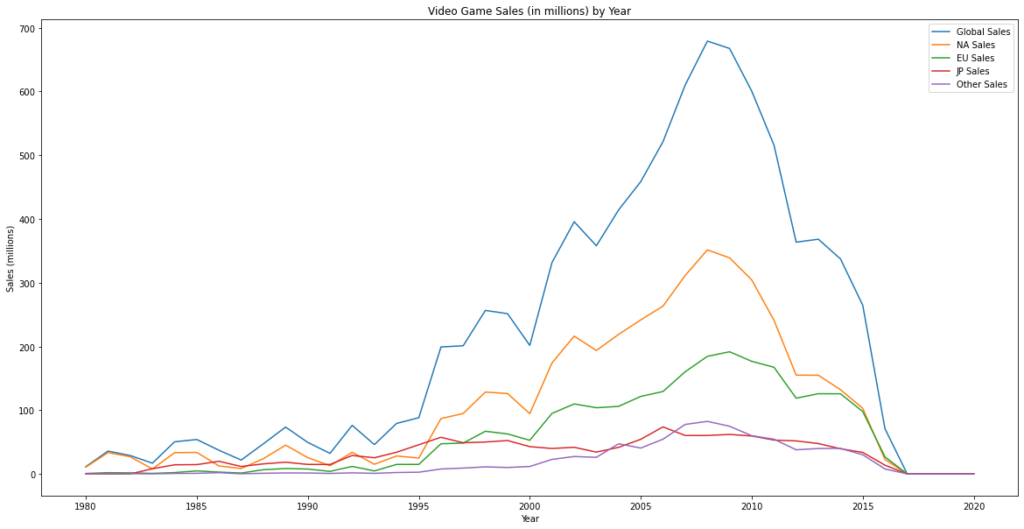
Looking at the line plot, we can simply infer that video game sales were most significant during the first decade of the 21^st century. After that, sales of video games have taken a dip.

Another interesting observation is that during the period 1990-1995, sales in Japan even superseded those of Europe and North America. To know the reason behind these numbers, an investigation needs to take place by considering the social or economic factors during that time. This investigation may produce some useful insights that the businesses may use to boost the sales in the region of Japan.

Genre Sales

To find the sales of games by genre, we need to calculate the cumulative values of sales for each genre in the dataset. To do this, we need to group by ‘genre’ and then take the summation of the values in each group.

Later, we can sort these values as per the global sales and extract the sales columns from the data frame:

genre_sales = vg_sales.groupby(['Genre']).sum().sort_values('Global_Sales', ascending=False)[['NA_Sales', 'EU_Sales', 'JP_Sales', 'Other_Sales', 'Global_Sales']]
genre_sales.head()

Output:

	             NA_Sales	EU_Sales	JP_Sales	Other_Sales	Global_Sales
Genre		
Action	861.77	516.48	158.65	184.92	1722.84
Sports	670.09	371.34	134.76	132.65	1309.24
Shooter	575.16	310.45	38.18	101.90	1026.20
Role-Playing	326.50	187.57	350.29	59.38	923.83
Platform	445.99	200.65	130.65	51.51	829.13

Since there are a total of 12 genres used in this dataset, we can a horizontal bar graph to visualize the sales for each genre in different regions of the world i.e., North America, Europe, Japan, Rest of the World:

genre_dum_values = np.arange(0, len(genre_sales.index)*2, 2)
bar_width = 0.3

plt.figure(figsize=(20,10))
plt.bar(genre_dum_values, genre_sales['Global_Sales'], width=bar_width, label='Global Sales')
plt.bar(genre_dum_values+bar_width, genre_sales['NA_Sales'], width=bar_width, label='NA Sales')
plt.bar(genre_dum_values+(bar_width*2), genre_sales['EU_Sales'], width=bar_width, label='EU Sales')
plt.bar(genre_dum_values+(bar_width*3), genre_sales['JP_Sales'], width=bar_width, label='JP Sales')
plt.bar(genre_dum_values+(bar_width*4), genre_sales['Other_Sales'], width=bar_width, label='Other Sales')
plt.xticks(genre_dum_values + (bar_width * (len(genre_sales.columns)-1)/2), labels=genre_sales.index)
plt.title('Video Game Sales (in millions) by Genre')
plt.xlabel('Genre')
plt.ylabel('Sales (millions)')
plt.legend()
plt.show()

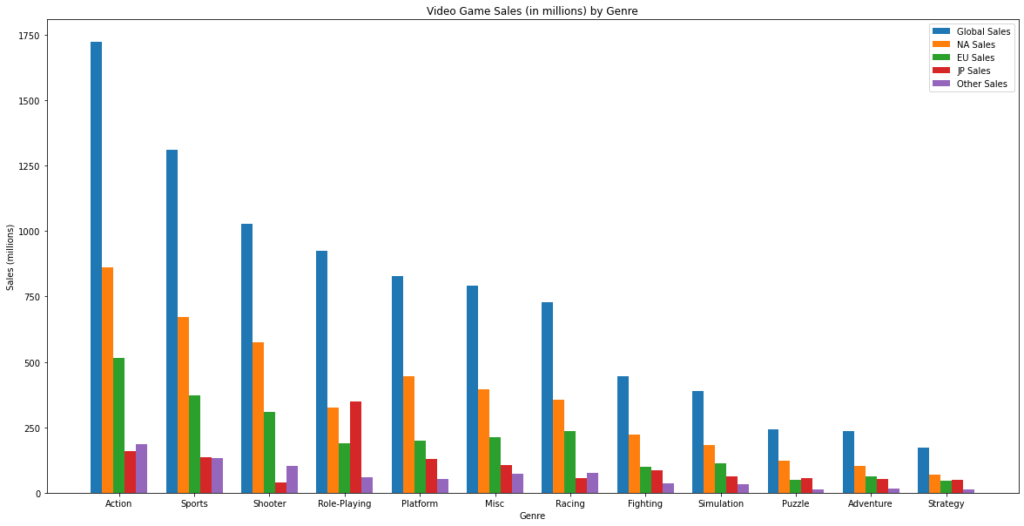
Looking at the above plot, we can extract the following insights for different genres of video games:

• Most of the game genres have majority of their sales in the region of North America and Europe.
• Action, Sports and Shooting games have got the majority market share. So, any startup looking to enter into market should firstly concentrate its effort on these genres
• Puzzle, Adventure and Strategy games have got the minority market share. So, these genres are to be avoided
• Role-Playing games have high sales potential in Japan. Any business looking to launch a game into this region is better off concentrating on this particular genre
• Japanese people do not seem to like Shooting and Racing games as is depicted in the sales. So, the companies are better off avoiding these genres when launching in the Japan region

Publisher Sales

To get the sales for each game publisher, we need to find the cumulative number of sales for each publisher by grouping the data frame using game publisher. The resulting data frame having the unique publisher at the index can be sorted as per the global sales:

publisher_sales = vg_sales.groupby(['Publisher']).sum().sort_values('Global_Sales', ascending=False)[['NA_Sales', 'EU_Sales', 'JP_Sales', 'Other_Sales', 'Global_Sales']]
publisher_sales.head()

Output:

	                    NA_Sales	EU_Sales	JP_Sales	Other_Sales	Global_Sales
Publisher		
Nintendo	815.75	418.30	454.99	95.19	1784.43
Electronic Arts	584.22	367.38	13.98	127.63	1093.39
Activision	426.01	213.72	6.54	74.79	721.41
Sony Computer Entertainment	265.22	187.55	74.10	80.40	607.28
Ubisoft	252.81	163.03	7.33	50.16	473.54

Now, we can draw a bar chart for the top 20 game publishers to extract useful insights from the visualization:

publisher_dum_values = np.arange(0, len(publisher_sales.index[0:20])*2, 2)
bar_width = 0.3
plt.figure(figsize=(20,10))
plt.bar(publisher_dum_values, publisher_sales['Global_Sales'][:20], width=bar_width, label='Global Sales')
plt.bar(publisher_dum_values+bar_width, publisher_sales['NA_Sales'][:20], width=bar_width, label='NA Sales')
plt.bar(publisher_dum_values+(bar_width*2), publisher_sales['EU_Sales'][:20], width=bar_width, label='EU Sales')
plt.bar(publisher_dum_values+(bar_width*3), publisher_sales['JP_Sales'][:20], width=bar_width, label='JP Sales')
plt.bar(publisher_dum_values+(bar_width*4), publisher_sales['Other_Sales'][:20], width=bar_width, label='Other Sales')
plt.xticks(publisher_dum_values + (bar_width * (len(publisher_sales.columns[:20])-1)/2), labels=publisher_sales.index[:20], rotation=270)
plt.title('Video Game Sales (in millions) by Publisher')
plt.xlabel('Publisher')
plt.ylabel('Sales (millions)')
plt.legend()
plt.show()

Looking at the above bar chart, following information could be extracted:

• Nintendo holds the biggest market share of the video games with most sales originating from North America followed by Japan, Europe and the rest of the world
• In the context of worldwide sales, Nintendo is followed by Electronic Arts, Activision, Sony and Ubisoft. Out of these four, only Sony has got the market share in Japan where the rest have the most sales generated from North America/Europe
• From the top 20 publishers, only 7 publishers have got the sales presence in Japan and the rest have almost NILL sales in that region. Seven publishers include Nintendo, Sony, Konami, Sega, Namco, Capcom and Square Enix. Other publishers are either failed to impress the Japanese gamers or not targeting the Japanese gaming market at all
• Namco and Konami have the most sales in Japan, even more than those of North America and Europe. This is an opposite of the trend followed by the other publishers. Both these publishers need to attract the gamers in North America and Europe as well to advance into the likes of Nintendo and Sony

Having analyzed the sales for a single feature, we will now the analyze the sales using a combination of two combines features of the video game dataset…

Platform Yearly Sales

To calculate yearly platform yearly sales, we need to group the data frame using both ‘platform’ and ‘year’ and then sum the sale values in a single group. This will result in a data frame having ‘year’ as the nested index whereas ‘platform’ will be the outer index:

platform_yearly_sales = vg_sales.groupby(['Platform', 'Year']).sum()[['NA_Sales', 'EU_Sales', 'JP_Sales', 'Other_Sales', 'Global_Sales']]
platform_yearly_sales.head()

Output:

		                          NA_Sales	EU_Sales	JP_Sales	Other_Sales	Global_Sales
Platform	Year					
2600	1980.0	10.59	0.67	0.0	0.12	11.38
      1981.0	33.40	1.96	0.0	0.32	35.77
      1982.0	26.92	1.65	0.0	0.31	28.86
      1983.0	5.44	0.34	0.0	0.06	5.83
      1984.0	0.26	0.01	0.0	0.00	0.27

Now we can draw yearly sales for top 12 platforms using the nested index representations of the data frame with the help of multiple line subplots in a single plot:

fig, ax = plt.subplots(3,4,figsize=(20,15))
for i in range(0,len(platform_sales[0:12].index)):
    row_index = int(i/4)
    col_index = i%4
    title_string = platform_sales.index[i] + ' Sales by Year'
    ax[row_index,col_index].plot(platform_yearly_sales.loc[platform_sales.index[i]].index, platform_yearly_sales.loc[platform_sales.index[i]]['Global_Sales'], label='Global Sales')
    ax[row_index,col_index].plot(platform_yearly_sales.loc[platform_sales.index[i]].index, platform_yearly_sales.loc[platform_sales.index[i]]['NA_Sales'], label='NA Sales')
    ax[row_index,col_index].plot(platform_yearly_sales.loc[platform_sales.index[i]].index, platform_yearly_sales.loc[platform_sales.index[i]]['EU_Sales'], label='EU Sales')
    ax[row_index,col_index].plot(platform_yearly_sales.loc[platform_sales.index[i]].index, platform_yearly_sales.loc[platform_sales.index[i]]['JP_Sales'], label='JP Sales')
    ax[row_index,col_index].plot(platform_yearly_sales.loc[platform_sales.index[i]].index, platform_yearly_sales.loc[platform_sales.index[i]]['Other_Sales'], label='Other Sales')
    ax[row_index,col_index].set_title(title_string)
    ax[row_index,col_index].legend()
fig.show()

Looking at the line plots, we can infer that yearly timeline is not the same for each platform. Some entered into the market early and left early, where as some enter the market late and are still sustaining.

Following are the some of the unique points which can be noted from the line plots:

• Most of the platforms have a gaussian-like yearly sale curve except DS, PC and GB sales. The sales of DS have only been recorded for the period 2005-2010, whereas the sales for PC and GB platforms are aberrant in nature during different periods
• For PSP, sales in Japan have exceeded for the period 2010-2014 compared to North America and Europe. A worrying sign, maybe!
• For PS2, sales in other countries are more than those of Europe and Japan for the period 2007-2010 which may indicate the increased marketing efforts of PS2 all over the world
• For PS4, sales in Europe are more than that of North America which may give a hint towards missing out on the massive revenue
• PC platform have more sales in Europe during the period 2005-2015 than North America, Japan or the rest of the world. This indicates the increased activity of the PC gamers during that period and may lead towards another likewise trend in the upcoming years

Genre Yearly Sales

To get yearly sales for different game genres, we will group our data using both ‘genre’ and ‘year’ columns and then take cumulative sum of sales for each individual group:

genre_yearly_sales = vg_sales.groupby(['Genre', 'Year']).sum()[['NA_Sales', 'EU_Sales', 'JP_Sales', 'Other_Sales', 'Global_Sales']]
genre_yearly_sales.head()

Output:

		                             NA_Sales	EU_Sales	JP_Sales	Other_Sales	Global_Sales
Genre	Year					
Action	1980.0	0.32	0.02	0.00	0.00	0.34
         1981.0	13.86	0.81	0.00	0.12	14.84
         1982.0	6.07	0.38	0.00	0.05	6.52
         1983.0	2.67	0.17	0.00	0.02	2.86
         1984.0	0.80	0.19	0.83	0.03	1.85

Now we can visualize the yearly sales of top 12 genres having the best global sales:

fig, ax = plt.subplots(3,4,figsize=(20,15))
for i in range(0,len(genre_sales.index)):
    row_index = int(i/4)
    col_index = i%4
    title_string = genre_sales.index[i] + ' Sales by Year'
    ax[row_index,col_index].plot(genre_yearly_sales.loc[genre_sales.index[i]].index, genre_yearly_sales.loc[genre_sales.index[i]]['Global_Sales'], label='Global Sales')
    ax[row_index,col_index].plot(genre_yearly_sales.loc[genre_sales.index[i]].index, genre_yearly_sales.loc[genre_sales.index[i]]['NA_Sales'], label='NA Sales')
    ax[row_index,col_index].plot(genre_yearly_sales.loc[genre_sales.index[i]].index, genre_yearly_sales.loc[genre_sales.index[i]]['EU_Sales'], label='EU Sales')
    ax[row_index,col_index].plot(genre_yearly_sales.loc[genre_sales.index[i]].index, genre_yearly_sales.loc[genre_sales.index[i]]['JP_Sales'], label='JP Sales')
    ax[row_index,col_index].plot(genre_yearly_sales.loc[genre_sales.index[i]].index, genre_yearly_sales.loc[genre_sales.index[i]]['Other_Sales'], label='Other Sales')
    ax[row_index,col_index].set_title(title_string)
    ax[row_index,col_index].legend()
fig.show()

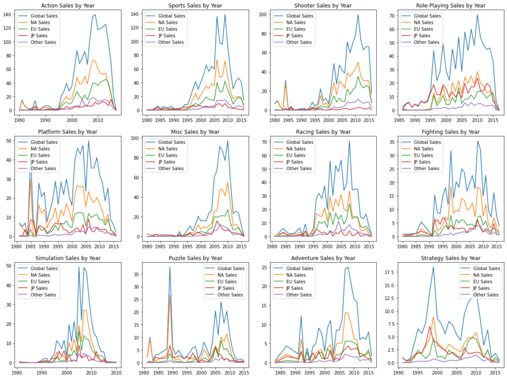
As expected, North America and Europe seem to lead the sales market for majority of the genres. However, there are some interesting findings which are highlighted below:

• For Role-Playing games, sales in Japan started out on top for the period 1985-2000, but these sales eventually got replaced by North America after the end of the 20^th century. This indicates the rising trend of role-playing games in North America as compared to Japan
• Majority of the genres have got uplift in their sales starting from 1995 onwards. However, Strategy and Adventure games seem to follow the opposite trend with their sales rising before the start of the 21^st century and declining later

Publisher Yearly Sales

To get yearly sales for each publisher, we need to group our data frame using both the publisher and the year columns. This will give us a data frame with nested index containing publisher as the outer index and the year as the internal index:

publisher_yearly_sales = vg_sales.groupby(['Publisher','Year']).sum()[['NA_Sales', 'EU_Sales', 'JP_Sales', 'Other_Sales', 'Global_Sales']]
publisher_yearly_sales.head()

Output:

		                      NA_Sales	EU_Sales	JP_Sales	Other_Sales	Global_Sales
Publisher	Year					
10TACLE Studios	2006.0	0.01	0.01	0.0	0.00	0.02
           2007.0	0.06	0.03	0.0	0.00	0.09
1C Company	2009.0	0.00	0.01	0.0	0.00	0.01
           2011.0	0.01	0.06	0.0	0.02	0.09
20th Century Fox Video Games	1981.0	1.27	0.07	0.0	0.01	1.35

We can now draw a plot to visualize the top 12 publisher with line plot indicating the yearly sales trend of each publisher:

fig, ax = plt.subplots(3,4,figsize=(20,15))
for i in range(0,len(publisher_sales.index[0:12])):
    row_index = int(i/4)
    col_index = i%4
    title_string = publisher_sales.index[i] + ' Sales by Year'
    ax[row_index,col_index].plot(publisher_yearly_sales.loc[publisher_sales.index[i]].index, publisher_yearly_sales.loc[publisher_sales.index[i]]['Global_Sales'], label='Global Sales')
    ax[row_index,col_index].plot(publisher_yearly_sales.loc[publisher_sales.index[i]].index, publisher_yearly_sales.loc[publisher_sales.index[i]]['NA_Sales'], label='NA Sales')
    ax[row_index,col_index].plot(publisher_yearly_sales.loc[publisher_sales.index[i]].index, publisher_yearly_sales.loc[publisher_sales.index[i]]['EU_Sales'], label='EU Sales')
    ax[row_index,col_index].plot(publisher_yearly_sales.loc[publisher_sales.index[i]].index, publisher_yearly_sales.loc[publisher_sales.index[i]]['JP_Sales'], label='JP Sales')
    ax[row_index,col_index].plot(publisher_yearly_sales.loc[publisher_sales.index[i]].index, publisher_yearly_sales.loc[publisher_sales.index[i]]['Other_Sales'], label='Other Sales')
    ax[row_index,col_index].set_title(title_string)
    ax[row_index,col_index].legend()
fig.show()

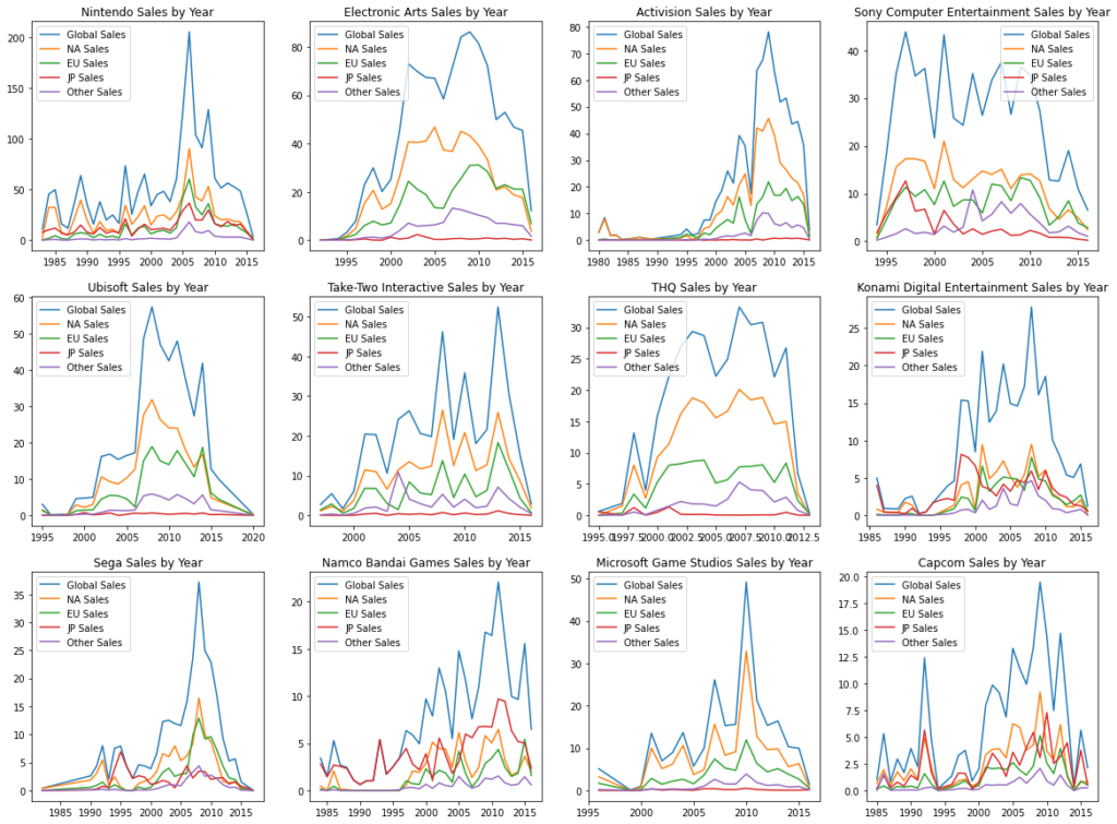
Looking at the above plot, we can visualize the normal trend of most publisher leading their revenue share from the North America and Europe. But let’s try to find some peculiarities in this visualization:

• Sony started off well with their sales in Japan from the period 1995-2000, but later lost their way in Japan. However, they made higher gains in rest of the world apart from North America and Europe
• Sega is also seen to be following the footsteps of Sony
• Contrary to most of the publishers, Konami was able to secure a tangible market of Japan in 1990 and sustain that market from thereon
• Namco Bandai did not only increase its revenue share in Japan but was also able to excel it more than North America and Europe, something which is a peculiar as far as the publishers are concerned. If any other publisher intends to advance their sales in Japan, they can follow what Namco Bandai has already done

Platform Genre Sales

To know about the sales each platform recorded for different genres, we need to group our main data frame (vg_sales) using both ‘Platform’ and ‘Genre’ and then take sum of sale numbers for each individual group.

platform_genre_sales = vg_sales.groupby(['Platform', 'Genre']).sum()[['NA_Sales', 'EU_Sales', 'JP_Sales', 'Other_Sales', 'Global_Sales']]
platform_genre_sales.head()

Output:

		                         NA_Sales	EU_Sales	JP_Sales	Other_Sales	Global_Sales
Platform	Genre					
2600	Action	24.63	1.47	0.0	0.21	26.39
         Adventure	0.38	0.02	0.0	0.00	0.40
         Fighting	0.72	0.04	0.0	0.01	0.77
         Misc	3.34	0.20	0.0	0.03	3.58
         Platform	12.38	0.72	0.0	0.16	13.27

We will now visualize the sales trend of different genres for top 12 platforms using individual bar charts in a single plot:

fig, ax = plt.subplots(2,2,figsize=(20,12))
bar_width=0.3
for i in range(0,len(platform_sales.index[0:4])):
    row_index = int(i/2)
    col_index = i%2
    title_string = platform_sales.index[i] + ' Platform game sales (in millions) by Genre'
    dum_values = np.arange(0,len(platform_genre_sales.loc[platform_sales.index[i]].index)*2,2)
    ax[row_index,col_index].bar(dum_values, platform_genre_sales.loc[platform_sales.index[i]]['Global_Sales'], width=bar_width, label='Global Sales')
    ax[row_index,col_index].bar(dum_values + bar_width, platform_genre_sales.loc[platform_sales.index[i]]['NA_Sales'], width=bar_width, label='NA Sales')
    ax[row_index,col_index].bar(dum_values + bar_width*2, platform_genre_sales.loc[platform_sales.index[i]]['EU_Sales'], width=bar_width, label='EU Sales')
    ax[row_index,col_index].bar(dum_values + bar_width*3, platform_genre_sales.loc[platform_sales.index[i]]['JP_Sales'], width=bar_width, label='JP Sales')
    ax[row_index,col_index].bar(dum_values + bar_width*4, platform_genre_sales.loc[platform_sales.index[i]]['Other_Sales'], width=bar_width, label='Other Sales')
    ax[row_index,col_index].set_xticks(dum_values + (bar_width * (len(platform_genre_sales.loc[platform_sales.index[i]].columns)-1)/2))
    ax[row_index,col_index].set_xticklabels(platform_genre_sales.loc[platform_sales.index[i]].index, rotation=45)
    ax[row_index,col_index].set_title(title_string)
    ax[row_index,col_index].set_ylabel('Sales (millions)')
    ax[row_index,col_index].legend()
fig.show()

fig, ax = plt.subplots(2,2,figsize=(20,12))
bar_width=0.3
for i in range(4,len(platform_sales.index[4:8])+4):
    row_index = int(i/2) - 2
    col_index = i%2
    title_string = platform_sales.index[i] + ' Platform game sales (in millions) by Genre'
    dum_values = np.arange(0,len(platform_genre_sales.loc[platform_sales.index[i]].index)*2,2)
    ax[row_index,col_index].bar(dum_values, platform_genre_sales.loc[platform_sales.index[i]]['Global_Sales'], width=bar_width, label='Global Sales')
    ax[row_index,col_index].bar(dum_values + bar_width, platform_genre_sales.loc[platform_sales.index[i]]['NA_Sales'], width=bar_width, label='NA Sales')
    ax[row_index,col_index].bar(dum_values + bar_width*2, platform_genre_sales.loc[platform_sales.index[i]]['EU_Sales'], width=bar_width, label='EU Sales')
    ax[row_index,col_index].bar(dum_values + bar_width*3, platform_genre_sales.loc[platform_sales.index[i]]['JP_Sales'], width=bar_width, label='JP Sales')
    ax[row_index,col_index].bar(dum_values + bar_width*4, platform_genre_sales.loc[platform_sales.index[i]]['Other_Sales'], width=bar_width, label='Other Sales')
    ax[row_index,col_index].set_xticks(dum_values + (bar_width * (len(platform_genre_sales.loc[platform_sales.index[i]].columns)-1)/2))
    ax[row_index,col_index].set_xticklabels(platform_genre_sales.loc[platform_sales.index[i]].index, rotation=45)
    ax[row_index,col_index].set_title(title_string)
    ax[row_index,col_index].set_ylabel('Sales (millions)') 
    ax[row_index,col_index].legend()
fig.show()

fig, ax = plt.subplots(2,2,figsize=(20,12))
bar_width=0.3
for i in range(8,len(platform_sales.index[8:12])+8):
    row_index = int(i/2) - 4
    col_index = i%2
    title_string = platform_sales.index[i] + ' Platform game sales (in millions) by Genre'
    dum_values = np.arange(0,len(platform_genre_sales.loc[platform_sales.index[i]].index)*2,2)
    ax[row_index,col_index].bar(dum_values, platform_genre_sales.loc[platform_sales.index[i]]['Global_Sales'], width=bar_width, label='Global Sales')
    ax[row_index,col_index].bar(dum_values + bar_width, platform_genre_sales.loc[platform_sales.index[i]]['NA_Sales'], width=bar_width, label='NA Sales')
    ax[row_index,col_index].bar(dum_values + bar_width*2, platform_genre_sales.loc[platform_sales.index[i]]['EU_Sales'], width=bar_width, label='EU Sales')
    ax[row_index,col_index].bar(dum_values + bar_width*3, platform_genre_sales.loc[platform_sales.index[i]]['JP_Sales'], width=bar_width, label='JP Sales')
    ax[row_index,col_index].bar(dum_values + bar_width*4, platform_genre_sales.loc[platform_sales.index[i]]['Other_Sales'], width=bar_width, label='Other Sales')
    ax[row_index,col_index].set_xticks(dum_values + (bar_width * (len(platform_genre_sales.loc[platform_sales.index[i]].columns)-1)/2))
    ax[row_index,col_index].set_xticklabels(platform_genre_sales.loc[platform_sales.index[i]].index, rotation=45)
    ax[row_index,col_index].set_title(title_string)
    ax[row_index,col_index].set_ylabel('Sales (millions)') 
    ax[row_index,col_index].legend()
fig.show()

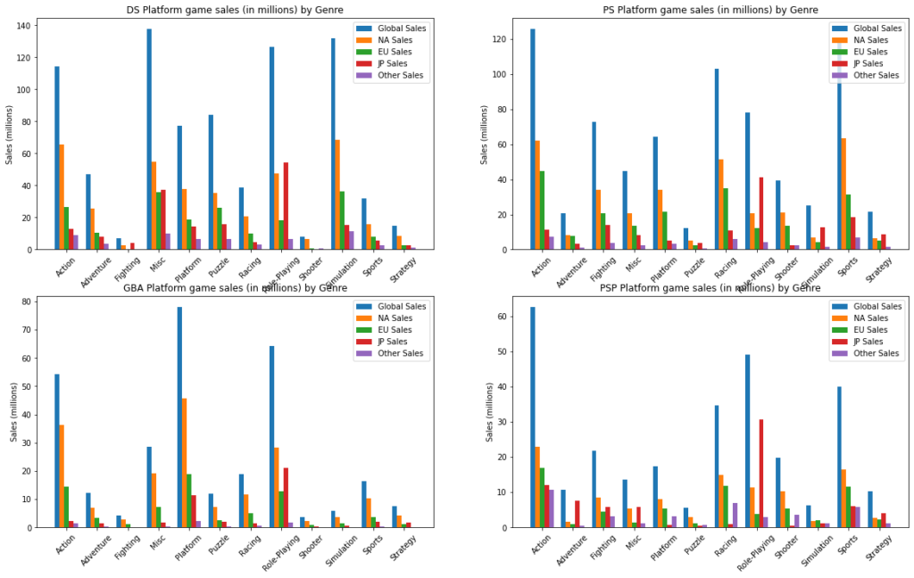
By closely analyzing the above 3 plots, we can generate some useful insights for business purpose. Some of the findings for each platform are described below:

• For PS2 platform, genres generating most revenue include action, sports, racing and shooting. For role-play and sports genres, Japan has the significant share in the total revenue
• For X360 platform, most sales are generated by shooting, action and sports games. Looking at the plot, it is evident that X360 is highly unpopular among the Japanese people and the owners might be missing a trick here
• PS3 platform has their most sales generated using Action, Shooting and Sports games. Apart from North America and Europe, PS3 has low share in the Japanese and the rest of the world market. So, a concentrated effort needs to be put in to increase sales in the low-sale regions
• Wii platform has almost 80% of their sales generated using Sports, Miscellaneous and Action based games. To raise their stakes in the market, they should look to launch a shooting or racing game preferably in the North America or Europe region
• DS platform seem to have generated most of the revenue using Role-Playing and Simulation games. More importantly, it is able to penetrate the Japanese market for almost all kind of games which is actually missing for other platforms
• PS platform tend to generate most sales from Racing, Sports, Action and Role-Playing games, but it follows in the footsteps of DS platform in that it has generated a chunk of its total sales from the Japanese market
• GBA platform has most of its sales recorded for Role-Playing and Action based games. Extremely low sales in the other genres could be costing sales all over the world
• PSP platform generates most of the sales using Action, Role-Playing and Sports games. The highest individual sale recorded for this platform is in Japan for role-playing games; a trend which others platform owners can follow to increase their market share in the Japanese market
• PS4 platforms tends to generate most revenue using Action, Sports and Shooting games. Other than that, it produces not much sales from other genres or from the Japanese market
• PC games generating most the revenue come from the genres of Shooting, Simulation, Strategy and Role-Playing. In fact, PC games are the only ones generating the highest revenue from the strategy games out of the top 12 platforms. Again, PC games have failed to attract the attention of Japanese gamers
• GB platform have the highest sales in Role-Playing games, primarily, because of their massive penetration in the Japanese market for the same genre. Other revenue generating genres include Puzzle and Adventure
• XB platform generates most of the sales using Action, Racing, Shooter and Sports games, but on the same time, fail to gather revenue from the Japanese market which could be costing a fortune to the owners

Conclusion

In this tutorial, we analyzed the sale data of video games and extracted useful insights which might help platform manufacturers and game publishers to plan their next game launch in a specific genre or a specific region including North America, Europe, Japan, and the rest of the world. The analysis revealed that most of the revenue was generated from the region of North America and Europe. Moreover, only a few publishers and game genres have got the massive sale numbers in Japan and control the overall gaming market there.

Hence, Japan presents a lucrative opportunity for any established business looking to increase its sales. Moreover, any startup aiming to enter the video game market should target North America and Europe with games based on popular genres i.e., sports, shooting, action and racing, etc.

Awais Naeem

He is the owner and founder of Embedded Robotics and a health based start-up called Nema Loss. He is very enthusiastic and passionate about Business Development, Fitness, and Technology. Read more about his struggles, and how he went from being called a Weak Electrical Engineer to founder of Embedded Robotics.

Follow him on Facebook, Twitter, LinkedIn

Sharing is Caring!